0x01 Introduction
Recently I’m working on visualization of flow velocity pulsation, it is necessary to draw a contour map of the distribution of the velocity pulsation intensity on the cross section. The Chart control provided by Winform does not provide the function of contour drawing. So I look up in Baidu for some information, and probably learned the steps of contour drawing, and I will share it with you here. The main idea is to divide the space region by Delauney triangles, and then contour trace after interpolation to draw contours and finally mark them.
0x02 Triangulation

Through spatial interpolation, we can easily obtain the sampling data of the locations near the sampling point. Common methods include natural adjacent interpolation, surface patches, quadrics, polynomial interpolation, spline curves, and Delauney triangles. This type of method has a wide range of applications in terrain data (DEM), meteorological data, finite element analysis, and grid generation.
- The triangulation assumes that V is a finite point set on a two-dimensional real number field, edge e is a closed line segment consisting of points in the point set, and E is a set of e. Then a triangulation T = (V, E) of the point set V is a plane graph G, which meets the conditions:
- Except for the endpoints, the edges in the plan do not contain any points in the point set.
No intersecting edges. - All faces in the plan view are triangular faces, and the collection of all triangular faces is the convex hull of the scattered point set V.
Delauney meshing is a special case of triangulation, which requires two principles to be met:
- Empty circle characteristics: Delaunay triangle network is unique (any four points cannot be co-circular), and no other points exist in the circumscribed circle of any triangle in the Delaunay triangle network.
- Maximum minimum angle characteristics: Among the possible triangles formed by the scattered point set, the triangle formed by Delaunay triangulation has the smallest angle. In this sense, Delaunay triangulation is the “closest to regular” triangulation. Specifically, it means that the diagonal of a convex quadrilateral is formed by two adjacent triangles. After the mutual exchange, the minimum angle of the six internal angles no longer increases.
Due to the above principles, Delayney triangulation has the following excellent characteristics:
- Closest: A triangle is formed with the nearest three points, and the line segments (edges of the triangle) do not intersect.
- Uniqueness: No matter where you start building in the region, you will end up with consistent results.
- Optimality: If the diagonals of the convex quadrilaterals formed by any two adjacent triangles are interchangeable, the smallest angle of the six internal corners of the two triangles will not become larger.
- The most regular: If the smallest angle of each triangle in the triangle net is arranged in ascending order, the value obtained by the arrangement of the Delaunay triangle net is the largest.
- Regionality: Adding, deleting and moving a vertex will only affect the adjacent triangles.
Shell with convex polygon: The boundary of the outermost layer of the triangular mesh forms a shell with a convex polygon.
0x03 Implementation on triangulation
There are various way to implement DELAUNEY Triangulation, here I will introduce the most original and simplest one – Lawson Algorithm.
Before we go futher, let me explain one terminology, LOP, which is abbreviation for Local Optimization Procedure, this is the core method of Lawson Algorithm.
If we are given 4 spatial point, we can make two different kinds of triangle net as follow. From the definition of DELAUNEY triangle net we know that the latter one is a DELAUNEY triangle net while the former one is a normal triangle net, with the help of LOP, we can transform the ordinary triangle net to DELAUNEY’s one. The basic approach is as follows:
- Combine two triangles with common edges into a polygon
- Check with the maximal empty circle rule to see if the 4th vertex is within the circumscribed circle of the triangle
- If yes, change the diagonal line, which is switching line BD to AC in this picture. After that, the processing of the local optimization process is completed.
Now that we acquire a basic knowledge on LOP, we can take a step further. Lawson’s Algorithm can be described in following procedure:
- Create a large triangle or polygon, enclose all the data points
- Insert a point into it, this point is connected to the three vertices of the triangle that contains it, and form three new triangles, and then perform empty circle detection on them one by one.
- At the same time, the local optimization process LOP designed by Lawson is used to optimize, that is to ensure that the triangle network formed is exchanged to ensure that the formed triangular network is a Delaunay triangular network.
0x04 Code and explaination
1 2 3 4 5 6 7 8 9 10 11 12 13 14 15 16 17 18 19 20 21 22 23 24 | subroutine triangulate input : vertex list output : triangle list initialize the triangle list determine the supertriangle add supertriangle vertices to the end of the vertex list add the supertriangle to the triangle list for each sample point in the vertex list initialize the edge buffer for each triangle currently in the triangle list calculate the triangle circumcircle center and radius if the point lies in the triangle circumcircle then add the three triangle edges to the edge buffer remove the triangle from the triangle list endif endfor delete all doubly specified edges from the edge buffer this leaves the edges of the enclosing polygon only add to the triangle list all triangles formed between the point and the edges of the enclosing polygon endfor remove any triangles from the triangle list that use the supertriangle vertices remove the supertriangle vertices from the vertex list end |
1 2 3 4 5 6 7 8 9 10 11 12 13 14 15 16 17 18 19 20 21 22 23 24 25 26 27 | input: vertices initialize vertices array create indices array (indices = new int[vertices.Count]) //indices array should be like {0,1,2,3,......,vertices.Count - 1} sort indices from small to big based on vertices's x coordinate value // can also be sorted by y value determine super triangle add super triangle to temp triangles push super triangle to triangles for each point in vertices // point iteration should be followed by sorted indices initialize the edge buffer for each triangle in temp triangles calculate the triangle circumcircle center and radius if the point lies on the right side of triangle circumcircle then this triangle is Delaunay triangle, save it to triangles delete this triangle in temp triangles continue else if the point lies on outside circumcircle then // this triangle is undetermined, do nothing here, I will explain it later continue else // which is inside the circumcircle // this triangle is not a Delaunay triangle add the three triangle edges to the edge buffer remove this triangle in temp triangles delete all duplicate edges generate new triangles via edges and point and save them to temp triangles combine triangles and temp triangles remove triangles which are related to super triangle end |
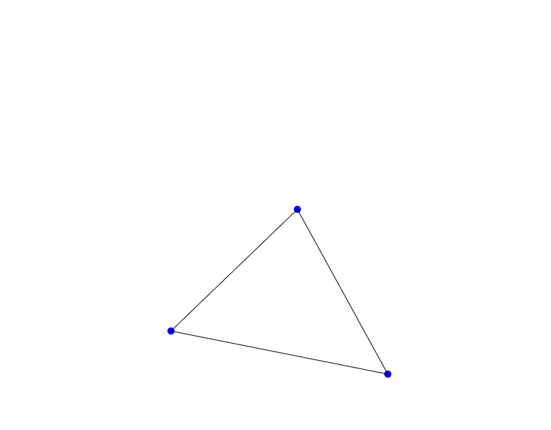
Aforementioned pseudocode maybe still too difficult to read, here I will introduce a 3 points illustration for better understanding to optimized version.
Firstly, we need to generate super triangle based on 3 points’s min max range, then save it to temp triangles
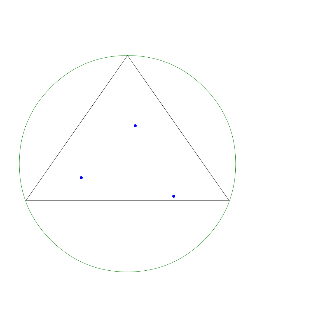
Secondly, iterate through 3 points, we will have the left one first, then iterate through temp triangles, here we will get the super triangle, we can know that this point lies in the circumcircle of super triangle, so add super triangle’s edge to edge buffer(edges) and delete the super triangle in temp triangles.
Thirdly, remove duplicate edges in edge buffer and generate new triangles by edge buffer and current point then save them to temp triangles.

Fouthly, now we have 3 triangles in temp triangles, we will go to the second point,clear edge buffer, create circumcircle and judge its relationship to the second point, in the following picture we can see that triangle 1 is Delaunay triangle because second point lie on the right outside of circumcircle 1, triangle 2 is unknown triangle because second point lie outside of circumcircle 2 and not on the right side of it, triangle 3 is not Delaunay triangle because the point lie inside of circumcircle 3, we will have to remove triangle 3 in temp triangles and add its edges to edges buffer, then generate new triangles with edges buffer and second point.
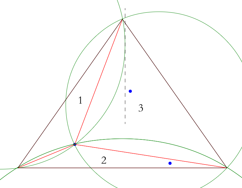
Fifthly, we will come to the last point, continue iteration through temp triangles, there should be 4 triangles in it, 3 new generated triangles and 1 unknown triangle. Triangle 1 is Delaunay, triangle 2 is unknown, triangle3 and triangle 4 should be removed from temp triangles and their edges should be added to edges buffer to build new triangles.
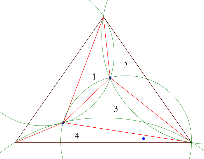
Finally, remove duplicate edges and build latest triangles then add them to temp triangles, since there’s no point left, we will come to the last stage, combine triangles and temp triangles, remove all triangle which is relevant to super triangle (triangles which have super triangle’s vertice), we will have the final Delaunay triangle list.